Behaviour of Revenue

We distinguish between two types of market situation in this situation

1) Perfectly competitive market

2) Imperfectly competitive market

The behaviour of Toal revenue, Average revenue and Marginal revenue will be different in the two types of market.

Relationship between TR, AR and MR under Perfect Competition

A firm under perfect competition is able to sell additional units of output at the ruling price. It is not required to reduce the price to sell more.

Reason:

As perfect competition is a market structure where there are large number of firms, so increase or decrease in production by any one firm do not affect in total supply in the whole market and also on price.

The collective force of demand and supply determines price in perfect competition which prevails in the market.

So each firm sells at the prevailing price (so do not reduce the price to sell more).

So firms are price taker and their demand curve is perfectly elastic.

Tabular Relationship between TR, AR and MR under Perfect Competition

Units of output (Q)	Price  ( P)	AR (TR / Q)		TR (P x Q)	MR (TRn- TRn-1)
1 2 3 4 5	10 10 10 10 10	10 10 10 10 10	10 20 30 40 50		10 – 0 = 10 20 – 10 = 10 30 – 20 = 10 40 – 30 = 10 50 – 40 = 10

Relation between average cost and marginal cost

There is an important relation between the average cost and marginal cost curves. The relation is shown in table and in graph.

Tabular representation

Units of Output	Total Cost	Marginal Cost	Average cost AC = TC / Q
0 1 2 3 4 5 6 7 8	10 20 28 34 38 42 48 56 72	- 10 8 6 4 4 6 8 16	∞ 20 14 11.3 9.5 8.4 8 8 9

Graphical representation

average cost

From the above table and graph following observations can be made between AC and MC

Marginal Cost

Marginal cost is the change in total cost when additional unit of output is produced.

As said by Ferguson “Marginal cost is the addition to total cost due to the addition of one unit of output.”

Symbolically,

MC_n = TC_n – TC_n-1 OR

MC = Change in total cost / Change in output

MC_n = Marginal cost of ‘n’ units of output

TCn = Total cost of ‘n’ units of output

TC_n-1 = Total cost of ‘n-1’ units of output

Tabular representation of calculating MC

Units of Output	Total Fixed        Cost	Total  Variable         Cost	Total Cost	Marginal Cost
0 1 2 3 4 5 6 7 8	10 10 10 10 10 10 10 10 10	0 10 18 24 28 32 38 46 62	10 20 28 34 38 42 48 56 72	- 10 8 6 4 4 6 8 16

Average Cost Curves

Average Cost is the cost per unit of output produced. It is also called unit cost of production.

Average cost = Total cost / Output

AC = TC / Q

Calculating AC when Total Cost is given

Units of Output	Total Cost	AC = TC/ Q
0 1 2 3 4 5 6	10 20 28 34 38 42 48	∞ 20 14 11.3 9.5 8.4 8

Corresponding to three types of total cost in the short run, there are three types of average cost:

1) Average Fixed cost

2) Average Variable cost

3) Average total cost

Average Total Cost is the sum total of average Fixed cost and average variable cost.i.e.

AC = AFC + AVC

Short Run Costs

Short run is the period of time during which some factors are fixed and some are variable.

Short run costs are divided into two components:

1) Fixed costs

2) Variable costs

Total Cost = Total fixed cost + Total variable cost

i.e. TC = TFC + TVC

Fixed Cost :

Fixed costs are the sum total of expenditure incurred by the producer on the purchase or hiring of fixed factors of production.

These are also called supplementary costs  or overhead costs or  indirect costs.

These costs do not change with the change of output, even when output is zero, fixed cost remains the same.

For example: In a shoes manufacturing firm, a machine is installed as a fixed factor.

If it can make 10 pair of shoes a day and that the cost of hiring the machine is Rs. 100 per day.

So Rs. 100 per day is the fixed cost that the producer has to incur even when no shoes is made in a day.

The fixed cost would remain Rs. 100 (between 0 to 10 shoes a day).

Stages of Production

The behaviour of output in terms of TP, AP and MP on account of increasing variable input is divided into three stages, as shown in the graph below:

Stages of Production

Stage I : Stage of increasing returns

1) Starts from the point of origin and continues till the AP is maximum at point A

2) TP is increasing throughout the first stage.

Till point M(point of infexion) increasing at increasing rate and after point M increasing at decreasing rate till point A.

3) MP rises first, reaches the maximum at point M and then it starts falling, but is positive throughout.

Till point M has the positive slope and after that negative slope.

Law of Variable Proportion

The law of variable proportion states that as more and more units of variable factors are applied to the given quantity of a fixed factor, the total product may increase at an increasing rate initially, but eventually it will increase at a diminishing rate.

Explaining the above law by taking an example:

A farmer is producing wheat, he has land as a fixed factor and labour as a variable factor.

Since land is a fixed factor, he can produce more of wheat only by using more and more of labour.

Will every additional unit of labour employed on the given land yield the same amount of additional output of wheat?

No, it can never happen. If MP (marginal product/additional output) of labour was to remain constant, then a country like India would have produced more and more of wheat using more and more of labour on the same piece of land. It would have never faced the problem of food.

So MP eventually dimnish.This is due to the fact that, there is some ideal ratio of factors of production.

Relation between TP/MP and AP/MP curves

1) Relation between Total product(TP) and Marginal Product(MP) 

We will explain the relation between TP and MP by the below graph:

marginal product

1) So long as  MP is increasing , TP is increasing at increasing rate.
MP is rising till point ‘b’ in the second graph and so is TP is increasing at increasing rate till point ‘a’ in the first graph.

Price Ceiling

In countries like India essentials of life, like certain food grains or life saving medicines, are often found to be extremely scarce.

Their prices are often found to be high. Poor population found it difficult to buy them. Such a situation often compels the government to intervene in the market with Price Ceiling. 

It means fixing a maximum price for a commodity which is generally much below the equilibrium market price.

Ceiling means maximum limit. Price ceiling means the maximum price of a commodity that the seller can charge from the buyers for a particular good and service. It is also termed as Maximum price Legislation.

Price Ceiling Policy

Let us understand the implication of price ceiling policy through the below graph.

Price Ceiling

DD and SS are the demand and supply curve respectively. OP is the equilibrium price and OQ is the equilibrium quantity. E is the point of equilibrium.

Time Element and Equilibrium Price

Equilibrium price is determined by the industry at that point where total demand is equal to total supply.

But, whether demand will have more effect or supply on the determination of the price, will depend on how much time will it take for the demand and supply to stabilize.

Importance of time element in the determination of price has been first examined by Dr. Marshall.

According to him, shorter the time period, greater will be the influence of demand in price determination and longer the period, greater will be the influence of supply on prices.

Marshall has divided the time elements into four periods:

1) Very short period or market period

2) Short period

3) Long period

4) Very long period

Very short period or market period

It is the time period during which supply of a commodity can be increased only up to the extent of its existing stock.

In case of perishable commodity which cannot be stored, supply becomes absolutely fixed or perfectly inelastic.

Some special cases of equilibrium

We have already explained the effects of change in demand and supply on the equilibrium price and quantity when demand and supply curves are normal slope, i.e. negatively sloping demand curve and positively sloping supply curve.

Let us consider how increase and decrease in demand affect equilibrium price in two exceptional situations:

1) When supply of the commodity is perfectly elastic        

2) When supply of the commodity is perfectly inelastic

When supply of the commodity is perfectly elastic

When supply curve is perfectly elastic i.e. supply curve is parallel to X axis, increase or decrease in demand  for a commodity does not cause any change in its price, equilibrium quantity tends to change. 

This is shown in the graph below:

perfectly elastic

E is the initial point of equilibrium when perfectly elastic supply curve(SS) intersect demand curve (DD). OP is the equilibrium price and OQ is the equilibrium quantity.

Forward shift in demand curve from DD to D₁D₁ leaves price of the commodity unchanged at OP. Equilibrium quantity increases from OQ to OQ₁.Equilibrium point shifts to E₁.

Backward shift in demand curve from DD to D₂D₂ leaves price of the commodity unchanged at OP. Equilibrium quantity decreases from OQ to OQ₂. Equilibrium point shifts to E₂.

Effect of Simultaneous changes in Demand and Supply

We have already discussed the effects of changes either in demand alone or in supply alone on the equilibrium price and quantity. But in reality changes in demand and supply take place simultaneously.  When demand changes, supply will also change as a consequence of that.

We will discuss below two situations of simultaneous changes in demand and supply :

a) Simultaneous Increase in Demand and Supply :

Simultaneous increase in demand and supply must cause increase in equilibrium quantity of the commodity.

But would there be any changes in price or not depends on whether demand increases more than, equal to, or less than supply.

So there can be three situations in this respect. As shown by the graphs below.

Change in Demand Supply and Market Equilibrium

We have already discussed the price determination of a commodity whose demand and supply curves are given, but generally demand and supply keeps on changing, resulting in shift in demand (factors like income, tastes and preferences etc.) and supply( change in technologies, input prices etc.) curves.

Let us now see the effect of change in demand and supply, on the equilibrium price and quantity.

Change in demand and Market Equilibrium

Change in demand has two aspects:

1) Increase in demand- demand curve shift to the right

2) Decrease in demand- demand curve shift to the left

Increase in demand:

demand supply

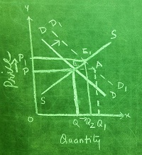
In the above diagram, DD and SS are the initial demand and supply curves. Equilibrium is struck at E, P and Q is the initial equilibrium price and quantity.

Determination of Market equilibrium Under Perfect Competition

Market equilibrium is a situation of the market in which demand for a commodity is exactly equal to its supply, corresponding to a particular price.
Thus, in a state of equilibrium, the market clears itself, as

Market demand = Market Supply

There is neither excess demand nor excess supply.
In this situation , the price that prevails in the market is called Equilibrium Price, Quantity supplied and demanded is called Equilibrium Quantity.

In a competitive market a single consumer or a single seller has no influence over the market price and so has no role to play in the determination of price.

Instead the price is determined in the competitive market through the interaction of market demand and supply.

How is the equilibrium price determined by the market forces of demand and supply?

Explanation through Table :

Price of X(apples) (Rs.)	Quantity Supplied (kg/week)	Quantity demanded (kg/week)	Market Position
5 4 3 2 1	50 40 30 20 10	10 20 30 40 50	Excess supply Excess supply Equilibrium Excess demand Excess demand

The above table shows as the price of commodity X falls, quantity demanded rises (law of demand)

and quantity supplied falls(law of supply).